Leaping into Lempel-Ziv Compression Schemes
Exploring one of the significant compression algorithms in an intuitive fashion

Hey everyone! In this blog, we're going to continue our discussion on data compression, but this time, we're diving into some real-world algorithms that make it all happen.
Here was my previous blog which builds the intuition behind compression:
A quick recap…
In the previous blog, we dove into the world of compression algorithms! We explored the fascinating idea that compressing data can, in some cases, actually make the file size bigger. We talked about how every compressed data set has a counterpart that expands when compressed. This is because compression relies on finding patterns within the data.
Idea behind a practical Compression Scheme
One way to deterministically achieve compression would be to have symbols for repeated chars or bits. Let’s take the example of the phrase to be or not to be. If we use a particular symbol X as a replacement for the to be part it will be encoded as: X or not X. This has reduced the number of symbols, hence we can say compression is achieved.
But wait, hold on a sec!! This raises a few questions:
What if we had the char
Xin the stream itself? Or a better question would be how to effectively differentiate between actual characters and symbols used as replacements?How will the decompressor know that
Xrefers toto be?
Solution #1: Let’s say our input is made up of 8-bit ASCII codes. Then in our compression scheme we can agree upon some kind of contract that after compression, the compressed data will be made up of 9-bit ASCII code instead. The decompressor will have to keep this information in mind. So, with 8 bit ASCII we have values from 0-255, with and additional bit we can have extra values from 256-511 that can be used for our symbols. This way we can very easily differentiate between symbols and input chars.
But wait, what kind of compression scheme is this, where we are taking the input is made up of 8-bit but the compressed data is made up of 9-bit? Won't that just increase the size of the data? Will compression be achieved at all?
That’s a really good question. Let’s tackle the 2nd question first and come back to this.
Solution #2: How will the decompressor know that X refers to to be? One approach would be to maintain a table/mapping for every symbol and what characters they represent. And the decompressor should also have this table/mapping information to refer to while performing the decompression.
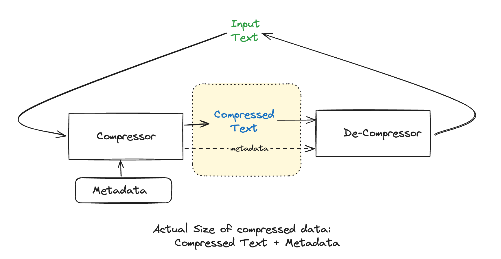
Here let me callout an important piece of information to keep in mind while developing compression schemes. When we compare compression algorithms we just can’t compare the compressed text with the original text. We need to take into account all the data that the decompressor needs, to be able to accurately decompress the compressed data to our original text (mind you we are still talking about lossless compression as mentioned in my earlier blog). So, in our case we will have to consider the compressed text + metadata (which can be the table/map that were talking) while comparing the performance of compression algorithms.
Now, let's tackle that tricky question.
From my previous blog we got an intuition that compression algorithms should be able to compress effectively, those inputs that are commonly used, at the expense of maybe expanding inputs which resembles random noise. So, when we use 9-bits or more in our compression scheme, we are hoping that with the extra 256 symbols we will be able to reduce the size so much that even with 9-bits we are able to get an effective compression. Let’s do that math with an example string: to be or not to be.
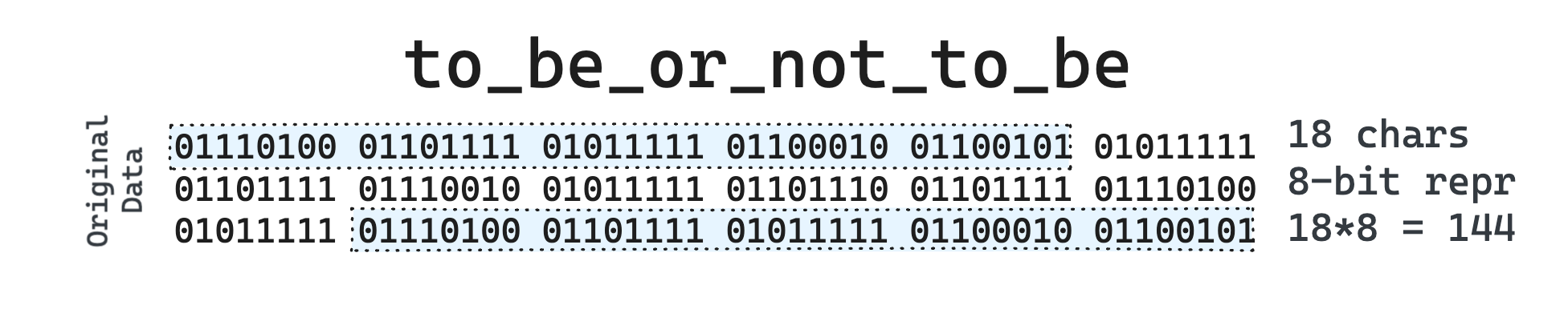
The original string has 18 chars, each char is of 8-bits i.e 18*8 = 144 bits in total.
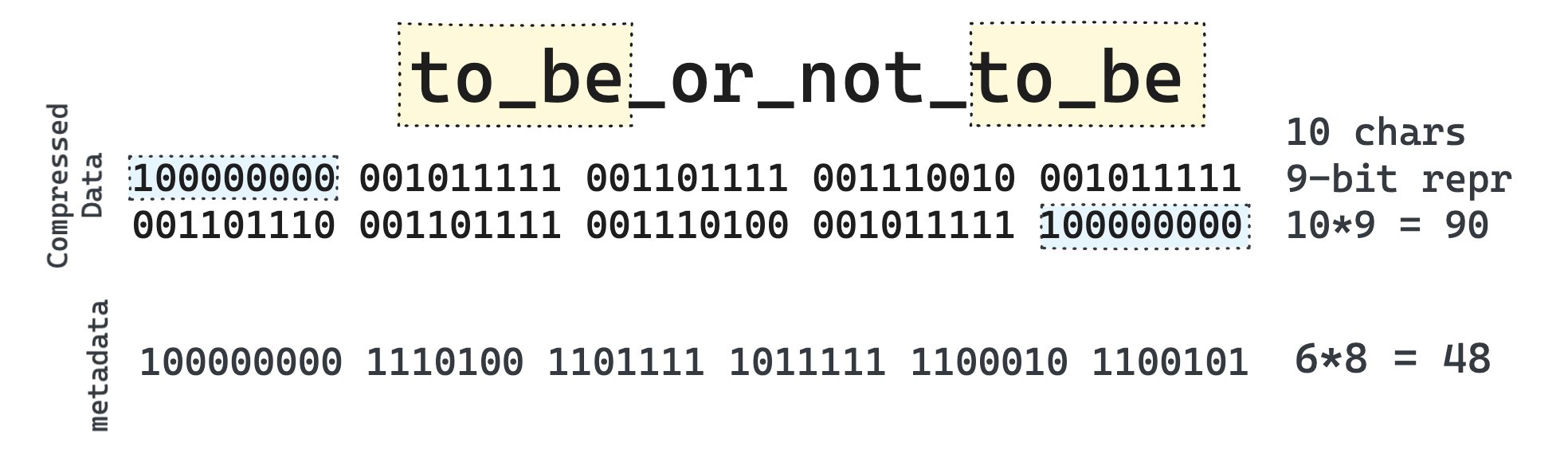
If we replace the to be with the symbol 256 (0b100000000) then the string itself gets compressed to just 10 symbols, with each symbol taking 9-bits according to our agreement i.e 10*9 = 90 bits.
But, also we need to take into account the additional mapping for the decompressor to know that symbol 256 refers to to be, that will take another 48 bits. So, effectively we have 90 + 48 bits = 138 bits and we achieve a compression ratio of 1.043. Although this compression is trivial, but this is a good example that supports our hypothesis.
Note: Trying to judge the compression schemes on smaller inputs is not ideal. Compression is all about saving space on large data. So, we should see if the compression scheme has the potential to scale with larger inputs. If the data to be compressed is itself very small, there is not much requirement to compress it anyways. But here, we will still stick to smaller inputs for easier understanding.
To draw some conclusion, to make a good compression algorithm, it needs to be able to find repeated patterns in the string and substitute them. But the tradeoff being, we have to somehow flow this information to the decompressor.
But is there any way we can make this even better? What if we can save the extra over-head to send the metadata to the decompressor?
Idea
One approach might be to traverse the input stream and build a dictionary simultaneously with all the information that we have so far. In other words, if the table/mapping can be built deterministically we don’t have to send that information to the decompressor and that will save us some extra overhead. The decompressor can use the same logic to build the table itself.
This is actually the hallmark of the LZ Scheme of Compression Algorithms. The LZ family of data compression algorithms trace back to the work of Abraham Lempel and Jacob Ziv, who published two influential papers in 1977 and 1978. These algorithms, LZ77 and LZ78, laid the groundwork for many variations that are still used today, including LZW, LZSS, and LZMA.
This article will focus on the LZW scheme. Terry Welch published it in 1984 (the W in the LZW) as a significant improvement to LZ78. The LZW algorithm quickly gained widespread use due to its efficiency and adaptability. It became the compression method of choice in the popular GIF image format. In 1985, Sperry Corporation (which had acquired Lempel and Ziv's employer) obtained a patent on LZW. Later, Unisys acquired Sperry and began enforcing licensing fees on the use of LZW in software. But developers weren’t happy with this but that hatred fueled the creation and adoption of other compression algorithms like DEFLATE (which is used in the gzip tool). But, the classic Unix command compress utilizes a modified version of the LZW algorithm.
It’s a little hard to explain the algorithm in a blog but I have given my best:
Getting hands dirty
Setup
The compressor and decompressor maintain a symbol table. The symbol table is initially populated with the first 256 ASCII characters. As we process the input string we will create new symbols and they will take the index 256 onwards. So, we can say symbol 256 is for to be and so on.
In the LZW compression algorithm, whenever we add something to the compressed data result, there must exist corresponding symbol in the symbol table.
We also have to maintain something called the Working String which stores a new symbol. At every step we either try to make the working string longer or add the current working string to the symbol table.
And, How do we build the working string? We use the Current Character while iterating the string. Once we add the current working string to the symbol table we reset the working string to just include the current character. So, effectively the working string is never empty except at the beginning of the compression.
Compression
Let’s consider an example string banana.
When we check if the working string is in the symbol table we append the current character at the end of it. Let’s define it as Augmented Working String (AWS) for easier understanding.
Let’s start with our first character: b.
Working String: "<empty>"
Current Character: "b"
Augmented Working String: “b”
Is AWS in the Symbol table? Yes, as we mentioned before, all the single character ASCII values are already in the table.
Now, the new working string becomes this augmented working string. And we don’t output anything in this step.
---
Let’s go to our next character: a.
Working String: “b”
Current Character: “a”
Augmented Working String: “ba”
Is AWS in the Symbol Table? No, currently we don’t have any extra symbols except the first 256 ASCII characters in the symbol table.
So, we will add this augmented working string in the symbol table with the next available index, which in this case is 256. So our symbol table now has this extra symbol:
symbol_table: {
    256: “ba”
}
At this point we will output the existing working string i.e “b”. So we got our first character in the compressed data.
---
Let’s go to our next character: n.
Working String: “a”
Current Character: “n”
Augmented Working String: “an”
Is AWS in the Symbol Table? No. So, we add it with the next available index i.e 257. Now our symbol table becomes:
symbol_table: {
    256: “ba”,
    257: “an”
}
And we output our current working string i.e “a”. So our compressed data is now ba.
---
Let’s go to our next character: a.
Working String: “n”
Current Character: “a”
Augmented Working String: “na”
Is AWS in the Symbol Table? No. So, we add it with the next available index i.e 257. Now our symbol table becomes:
symbol_table: {
    256: “ba”,
    257: “an”,
    258: “na”
}
And we output our current working string i.e “n”. So our compressed data is now ban.
---
Our next character: n.
Working String: “a”
Current Character: “n”
Augmented Working String: “an”
Is this in the Symbol Table? Well yes !! It’s index is 257. So, we move to our next step.
---
Our next character: a.
Working String: “an”
Current Character: “a”
Augmented Working String: “ana”
Is this in the Symbol Table? No. So, we add it with the next available index i.e 259. Now our symbol table becomes:
symbol_table: {
    256: “ba”,
    257: “an”,
    258: “na”,
    259: “ana”
}
And we output our current working string i.e “an” in fact the index for this symbol. So our compressed data is now ban<257>.
And our working string for the next iteration is “a”.
This is interesting to see that with this algorithm, we are even building up on the symbols that we already saw previously, in the hope that if it occurs again we can use this new symbol. This shows how compression schemes like this can benefit from repeated patterns in long input.
Now we are done with the input character, but we still have some data left in the working string. So, we need to flush them to the compressed data, so it becomes: ban<257>a.
As you can see we were building the symbol table as we were traversing the input. Another good observation is that we solved the problem of what a symbol represents. In the compressed string where we used 257 as a replacement for an; the substring an already exists in the string before the symbol has been used.
Decompression
For decompression the important objective is to build the symbol table by the time it reaches the symbol, so that it can use the substitution.
So, if the decompressor follows the same logic, by the time it reaches the symbol 257 it should be able to learn that 257 represents the character “an”. Let’s go through the decoding process too.
Now, we have the compressed data ban<257>a.
The logic to fill the symbols table remains the same.
Let’s go to the first symbol: b.
Working String: “<empty>”
Current character: “b”
Augmented working string: “b”
Since we already have the symbol in the table, we will continue and we can simply output the decompressed result b.
---
Next, our symbol is a.
Working String: “b”
Current Character: “a”
Augmented Working String: “ba”
We don’t have it in the symbol table so we will insert it:
symbol_table: {
    256: “ba”
}
And we will append “a” to the decompressed result: ba.
---
Our next symbol is n.
Working String: “a”
Current Character: “n”
Augmented Working String “an”
We don’t have it in the symbol table so we will insert it:
symbol_table: {
    256: “ba”,
    257: “an”
}
And we will append “n” to the decompressed result and it will be ban.
---
Next our symbol is 257 .
As soon as we come across a symbol we check if there is any substitution, and it does. We have “an” for 257. So, instead we will replace 257 with “an”. And treat each char individually like we were doing so far.
---
So, the next symbol is a (from the "an").
Working String: “n”
Current Character: “a”
Augmented Working String “na”
We don’t have it in the symbol table so we will insert it:
symbol_table: {
    256: “ba”,
    257: “an”,
    258: “na”
}
And we will append “a” to the decompressed result and it will be bana.
---
Then our next symbol will be n (We will still have a “n” from the substitution we performed earlier)
Working String: “a”
Current Character: “n”
Augmented Working String “an”
We have the symbol in the table, so we will continue with that augmented working string.
And we will append n to the decompressed result and it will be banan.
---
Now our final symbol is a.
Working String: “an”
Current Character: “a”
Augmented Working String “ana”
We don’t have it in the symbol table so we will insert it:
symbol_table: {
    256: “ba”,
    257: “an”,
    258: “na”,
    259: “ana”
}
Finally we will have our decompressed result: banana.
Also notice how we arrived at the same symbol table that we saw during the compression process. This is the beauty of the LZW compression algorithm.
Edge Case :)
But there is a small caveat !! Try to follow this same algorithm to compress the string another_banana and then decompress it. While compression you won’t find any issue and if you do it correctly you should get another b<256><265> as the compressed data. But there will be a small edge case when you perform the decompression.
But it can be resolved with a little trick.
Conclusion
"The art of compression is the art of finding patterns."
That was all for this blog. While LZW marked a significant milestone in compression algorithms, it's important to note that data compression continues to evolve. Modern techniques often combine LZW with other algorithms or use more sophisticated dictionary-building mechanisms to achieve even higher compression rates. Just like Google’s DeepMind AI AlphaDev found “faster” sorting algorithms, maybe someday they will come up with better and more efficient compression algorithms, until then let’s add more creativity to this field.